Creating a model fitting datakit
In this tutorial, we’ll explore a practical example of creating a model fitting datakit.
By the end, we’ll have created a datakit that can fit a linear or quadratic
model to an x/y input dataset using scipy. We’ll add a view to graph the
resulting fit curve against the data, and use relationships to handle
different parameters for each model.
Creating a new datakit
First, we need to create a new datakit:
dk new modelfitcd modelfit-datakitCreating the algorithm configuration
Next, we will need to put together an algorithm configuration for our model fitting algorithm.
Open up modelfit/algorithm.json and replace its contents with the following
configuration:
{ "name": "modelfit", "title": "Model fitting example", "description": "A simple model fitting algorithm demonstrating relationships", "profile": "datakit-algorithm", "code": "algorithm.py", "container": "opendatastudio/python-run-base:latest", "signature": { "inputs": [ { "name": "data", "title": "Data", "description": "Input data to fit to model", "type": "resource", "profile": "tabular-data-resource", "null": false, "default": { "resource": "data" } }, { "name": "model", "title": "Model", "description": "The model to use for fitting", "type": "string", "null": false, "enum": [ { "title": "Linear", "value": "linear" }, { "title": "Quadratic", "value": "quadratic" } ], "default": { "value": "linear" } }, { "name": "inputParams", "title": "Model", "description": "The input fit parameters", "type": "resource", "profile": "tabular-data-resource", "null": false, "default": { "resource": "inputParams" } } ], "outputs": [ { "name": "outputParams", "title": "Fit", "description": "The optimised fit parameters", "type": "resource", "profile": "tabular-data-resource", "null": true, "default": { "resource": "outputParams" } }, { "name": "fit", "title": "Fit", "description": "The optimised fit curve", "type": "resource", "profile": "tabular-data-resource", "null": true, "default": { "resource": "fit" } } ] }}This configuration defines three inputs: data, model and inputParams.
data and inputParams are tabular data resources, defining the input data
table and input parameter table respectively. model is a string that can take
one of two values: “linear” or “quadratic”. This tells the algorithm which model
we want to fit.
Similarly, we’ve defined two tabular resource outputs: outputParams and fit.
These are the output parameter table containing optimised parameter values, and
the calculated optimised fit curve.
Writing the algorithm
We want to create an algorithm that will take our input data and parameters, and
fit it to the selected model. Replace the code in modelfit/algorithm.py with
the following:
import pandas as pdfrom typing import TypedDictfrom scipy.optimize import curve_fit

class Output(TypedDict):    outputParams: pd.DataFrame    fit: pd.DataFrame

# Fit model functions

def linear(x, a, b):    """Linear fit model"""    return a * x + b

def quadratic(x, a, b, c):    """Quadratic fit model"""    return a * x**2 + b * x + c

# Main algorithm function

def main(data: pd.DataFrame, model: str, inputParams: pd.DataFrame) -> Output:    """Fit a linear or quadratic model to some data"""
    params, _ = curve_fit(        f=globals()[model],  # Call the global function named "model"        xdata=data.index,        ydata=data["y"],        p0=inputParams["init"],    )
    # Transform curve_fit output into expected output table format    names = ["a", "b", "c"]    table = [[name, param] for name, param in zip(names, params)]    outputParams = pd.DataFrame(        table,        columns=["name", "value"],    )
    # Calculate the optimised fit curve    fit = data.copy(deep=True)    fit["y"] = globals()[model](fit.index, *params)
    return {        "outputParams": outputParams,        "fit": fit,    }
Let’s go through this section-by-section:
# Fit model functions

def linear(x, a, b):    """Linear fit model"""    return a * x + b

def quadratic(x, a, b, c):    """Quadratic fit model"""    return a * x**2 + b * x + c
First, we define the fit model functions. These are the functions we will be
fitting to our data. They take the format expected by the scipy
curve_fit
function - a list of x values as the first argument, and then each individual
fit parameter as a separate argument.
def main(data: pd.DataFrame, model: str, inputParams: pd.DataFrame) -> Output:    """Fit a linear or quadratic model to some data"""
    params, _ = curve_fit(        f=globals()[model],  # Call the global function named "model"        xdata=data.index,        ydata=data["y"],        p0=inputParams["init"],    )
Next, we define the main algorithm function, which will be executed when the algorithm runs.
Here we use the scipy
curve_fit
function to optimise our chosen model.
The f argument specifies the function we want to use to fit the data: in our
case, it is chosen by the value of model algorithm variable which will either
be linear or quadratic. This will call the relevant fit model function
defined above when the algorithm is run.
xdata and ydata are simply the respective input data columns.
And p0 is an array of initial parameter guesses that are passed in via the
inputParams resource.
# Transform curve_fit output into expected output table format names = ["a", "b", "c"] table = [[name, param] for name, param in zip(names, params)] outputParams = pd.DataFrame( table, columns=["name", "value"], )Next, we do some data munging to transform the output of curve_fit into the
tabular format that our outputParams resource expects.
    # Calculate the optimised fit curve    fit = data.copy(deep=True)    fit["y"] = globals()[model](fit.index, *params)
    return {        "outputParams": outputParams,        "fit": fit,    }
And finally, we calculate the fit curve using the parameters returned by
curve_fit, and return our output data as per the outputs defined in the
algorithm configuration.
Creating resources
Before we can run our new algorithm, we need to create the resources it expects
as inputs and outputs: data, inputParams, outputParams and fit.
Create the resources directory:
mkdir modelfit/resourcesAnd create the following resource files:
Data
{ "name": "data", "title": "Data", "description": "Data to fit to model", "profile": "tabular-data-resource", "schema": { "primaryKey": "x", "fields": [ { "name": "x", "title": "X", "unit": "", "type": "number" }, { "name": "y", "title": "Y", "unit": "", "type": "number" } ] }, "data": []}This configuration specifies that we can accept a two column table with the column names “x” and “y” as input.
Input parameters
{ "name": "inputParams", "title": "Input parameters", "description": "Fit parameter initial guesses", "profile": "tabular-data-resource", "schema": { "primaryKey": "name", "fields": [ { "name": "name", "title": "Name", "description": "The name of the parameter", "type": "string" }, { "name": "init", "title": "Initial value", "description": "The initial guess for the parameter value", "type": "number", "unit": "" } ] }, "data": [ { "name": "a", "init": 3 }, { "name": "b", "init": 10 } ]}This specifies that we can accept our input parameters in a two-column table format. Our table is pre-populated with rows named “a” and “b” representing individual initial parameter guesses.
Output parameters
{ "name": "outputParams", "title": "Output parameters", "description": "Optimised parameter values", "profile": "tabular-data-resource", "schema": { "primaryKey": "name", "fields": [ { "name": "name", "title": "Name", "description": "The name of the parameter", "type": "string" }, { "name": "value", "title": "Optimised value", "description": "The optimised parameter value", "type": "number", "unit": "" } ] }, "data": [ { "name": "a", "value": null }, { "name": "b", "value": null } ]}Similar to inputParams, this specifies that we expect our output parameters to
be returned in a two-column table format. Our table is pre-populated with rows
named “a” and “b” representing individual optimised parameter outputs.
Fit
{ "name": "fit", "title": "Fit", "description": "The optimised fit curve", "profile": "tabular-data-resource", "schema": { "primaryKey": "x", "fields": [ { "name": "x", "title": "X", "unit": "", "type": "number" }, { "name": "y", "title": "Y", "unit": "", "type": "number" } ] }, "data": []}Similar to data, this specifies that we expect the calculated fit curve to be
output as a two column table with the column names “x” and “y”.
Adding input data
In order to run our algorithm, we need some test data. Pase the following into
data/modelfit.csv:
x,y0,0.34662361677399291,-0.4235315107624122,0.83881001954226793,2.9480000204777744,2.451676777777865,5.47664195524636456,4.8793233258853097,8.258761723473888,6.4426493545180419,10.1781629910989910,10.63827575297223211,10.3965503210973212,13.75275394389059613,12.87166064889421314,15.10522537094251715,13.08213503855560216,17.01213413269377717,15.06809087671543418,16.35653781069000719,20.825401723837388Running the algorithm
Now that we’ve created our algorithm configuration, algorithm code, and our input and output resources, we are ready to run the algorithm.
Initialise the default run:
dk initLoad the input data:
dk load data data/modelfix.csvAnd execute the run:
dk runOnce our algorithm finishes running, we can then view our outputs:
dk show outputParamsdk show fitCreating a graph visualisation
In order to be able to analyse whether our fit was a good one, we need to be able to graph the calculated fit curve.
We can create a graph visualisation by defining a view on our datakit.
First, create a views directory under the algorithm folder:
mkdir modelfit/viewsNow we can write a view configuration for our fit graph:
{ "name": "fitGraph", "specType": "matplotlib", "specFile": "fitGraph.py", "container": "opendatastudio/python-run-base:latest", "resources": ["data", "fit"]}Here we are telling our datakit that we want to use a matplotlib script,
fitGraph.py, to generate this view, and we want to execute this graph script
in the python-run-base container.
Now we can create our graph script:
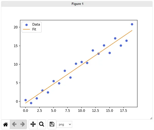
import pandas as pdimport matplotlib.pyplot as pltfrom matplotlib.figure import Figure

def main(data: pd.DataFrame, fit: pd.DataFrame) -> Figure:    plt.scatter(data.index, data["y"], label="Data", color="royalblue")    plt.plot(fit.index, fit["y"], label="Fit", color="darkorange")    plt.legend()
    # Return current figure    return plt.gcf()
Now we can execute the view script and generate the graph. Run the following command:
dk view fitGraphThis command will execute our graph script in the python-run-base container,
and then serve the resulting graph on a webpage for you to view.
In your browser, navigate to http://localhost:8988.
You should see the following:
Using relationships to accept an extra parameter
Introduction to relationships
You may have noticed earlier that in our quadratic model fit function
definition, we need an extra input parameter - c. However, this parameter
isn’t specified anywhere in our algorithm configuration or parameter resources.
In order to fit to a quadratic model, we need a way to dynamically add an extra
parameter whenever the value of the model algorithm variable is set to
quadratic.
We can do this using relationships. Relationships in a datakit describe relationships between variables. Whenever a variable changes, the CLI checks if there are any relationships that apply to that variable value, and if so updates any associated variables to the required values.
Relationships are defined in the algorithm directory under
modelfit/relationships.json.
Creating relationships
In order to add an extra parameter whenever the value of model is set to
quadratic, we need to write two relationship rules. Create the
modelfit/relationships.json file and write the following rules:
{ "name": "relationships", "title": "Relationships", "descriptions": "Relationship rules for model fit algorithm inputs and outputs", "profile": "datakit-relationships", "algorithm": "modelfit", "relationships": [ { "source": "model", "rules": [ { "description": "Linear model parameter defaults", "type": "value", "values": ["linear"], "targets": [ { "name": "inputParams", "type": "resource", "data": [ { "name": "a", "init": 3 }, { "name": "b", "init": 10 } ] }, { "name": "outputParams", "type": "resource", "data": [ { "name": "a", "value": null }, { "name": "b", "value": null } ] } ] }, { "description": "Quadratic model parameter defaults", "type": "value", "values": ["quadratic"], "targets": [ { "name": "inputParams", "type": "resource", "data": [ { "name": "a", "init": 3 }, { "name": "b", "init": 10 }, { "name": "c", "init": 5 } ] }, { "name": "outputParams", "type": "resource", "data": [ { "name": "a", "value": null }, { "name": "b", "value": null }, { "name": "c", "value": null } ] } ] } ] } ]}Breaking down the relationship configuration
In this relationship configuration, we are specifying that our source variable
is model. This means that we want to execute a set of rules whenever this
variable changes.
... "relationships": [ { "source": "model", "rules": [ ... ] } ]Each source variable can have any number of rules associated with it.
Each individual rule applies to a set of values of the source variable specified
in values. Whenever the source variable matches one of these values, the
associated rule will be executed.
... "relationships": [ { "source": "model", "rules": [ { ... "values": [ "linear" ], "targets": [ ... ] } ] } ]We can specify which associated variables we want to update when a rule is
triggered in targets. For example, below we are targeting the resource
inputParams. Whenever our source variable model is updated to the value
linear, we set the inputParams resource data to the specified values.
{ ... "relationships": [ { "source": "model", "rules": [ { "values": [ "linear" ], "targets": [ { "name": "inputParams", "type": "resource", "data": [ { "name": "a", "init": 3 }, { "name": "b", "init": 10 } ] } ...Putting it all together
Putting it all together, the above relationship configuration is doing the following:
- Whenever the
modelvalue is updated tolinear, it updates the input and output parameter resources to contain two variables -aandb. - Whenever the
modelvalue is updated toquadratic, it updates the input and output parameter resources to contain three variables -a,bandc.
In this way, we can dynamically handle a different number of parameters depending on the fit model chosen.
Running the algorithm again
Let’s test this out by running the algorithm again. Check the current parameter values:
dk show inputParams╭────────┬────────╮│ name │ init │├────────┼────────┤│ a │ 3 │├────────┼────────┤│ b │ 10 │╰────────┴────────╯Now let’s set the model to quadratic:
dk set model quadraticAnd check the parameter values again:
dk show inputParamsYou should see the following:
╭────────┬────────╮│ name │ init │├────────┼────────┤│ a │ 3 │├────────┼────────┤│ b │ 10 │├────────┼────────┤│ c │ 5 │╰────────┴────────╯As you can see, an extra parameter called c has been added.
Now we can run the algorithm and view the optimised parameters:
dk rundk show outputParams╭────────┬─────────────╮│ name │ value │├────────┼─────────────┤│ a │ -0.00663661 │├────────┼─────────────┤│ b │ 1.15614 │├────────┼─────────────┤│ c │ -0.838431 │╰────────┴─────────────╯And have a look at our resulting fit curve:
dk view fitGraph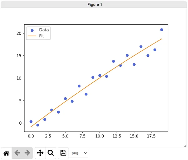
Congratulations, you’ve written and executed your own model fitting datakit.